Tuesday Analysis
John Clements and Jingjing Li 7/1/2021
Introduction
This project aims at analyzing and creating predictive models on “Bike
Sharing Dataset” at “UCI Machine Learning
Repository”
Where core data set is related to two-year log (2011, 2012) from Capital
Bikeshare system, Washington D.C. The data set mainly contains
information about the weather on a given day, when the day was (date,
season, month, and year), and whether the day was a holiday or working
day as well as bike rental counts including casual, registered riders
and total number of bike rentals (cnt).
In our study the total number of rentals on a given weekday (here
Tuesday) will act as the response, which makes more sense for bike
rental business compared to only the casual or the registered .
Explanatory variables comprise the weather variables, the season, and
the year. The weather related variables are temp (normalized
temperature), hum (normalized humidity), windspeed (normalized wind
speed), and weathersit. The variable weathersit is a factor going
from 1 to 4, with 1 being nice weather and progressing to 4, which
covers severe weather conditions. The season variable is a factor for
the four seasons, and yr is the year.
We analyze the data using plots and tables to see the distribution of
bike rentals, the weather situation of different seasons and construct
different models (two linear and two tree models) to predict bike rental
numbers affected by season, yr and weather situations represented by
temp,hum andwindspeed, compare those models and identify the best
one.
The main steps includes:
- load in the required packages
- read in the data and subset for Tuesdays and split into training and testings sets
- do exploratory analysis through summary statistics and data visualization
- evaluate models in repeated k-folds cross-validation (CV)
- evaluate the models on the withheld testing data
Now let’s get started by reading in loading the required packages.
library(readr)
library(tidyverse)
library(cowplot)
library(caret)
library(rmarkdown)
Reading in and Subsetting the Data
Before doing any analysis, we need to read in the daily bike-share data and subset for all the Tuesdays in the data set.
# Read in the daily data set.
bikeDay <- read_csv("./Bike-Sharing-Dataset/day.csv")
bikeDay <- filter(bikeDay, weekday == params$weekday)
Some of the variables, namely, season, mnth, holiday,
workingday, and weathersit are categorical, but are stored
numerically. Before proceeding with the analysis, we are converting them
to factor data types.
# Convert categorical variables stored numerically to factors.
bikeDay <- bikeDay %>%
  mutate(season = factor(ifelse(season == 1, "Spring",
                                ifelse(season == 2, "Summer",
                                       ifelse(season == 3, "Fall",
                                              "Winter"))),
                         levels=c("Spring", "Summer", "Fall", "Winter")),
         mnth = factor(mnth, levels=1:12),
         holiday = factor(holiday, levels=c(0, 1)),
         workingday = factor(workingday, levels=c(0, 1)),
         weathersit = ordered(weathersit, levels=c(1, 2, 3, 4))
         )
With that done, we can split the two data sets into training and testing sets for predictive modeling.
# Set a random seed for reproducibility.
set.seed(10)

# Set the proportion of observations to use for training models.
trainProp <- 0.7

# Get indexes for the training and testing subsets of the daily data.
trainIndexes <- sample(1:nrow(bikeDay),
                          size=nrow(bikeDay)*trainProp)
testIndexes <- setdiff(1:nrow(bikeDay), trainIndexes)
# Use the indexes to separate the training and testing sets of the daily data.
bikeTrain <- bikeDay[trainIndexes, ]
bikeTest <- bikeDay[testIndexes, ]
With our data sets created, we can now begin exploring the data.
Data Exploration
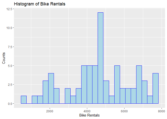
Let’s begin our exploration with a histogram of the number of bike rentals in a day for all the Tuesdays in the data to get an idea of the distribution.
# Create a histogram of bike rentals in a day.
plot1 <- ggplot(bikeTrain, aes(x=cnt)) +
  geom_histogram(bins=25, color="blue", fill="lightblue") +
  xlab("Bike Rentals") +
  ylab("Counts") +
  ggtitle("Histogram of Bike Rentals")

plot1

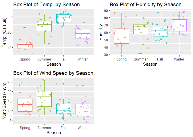
Next, let’s examine the numeric variables related to weather: temperature, humidity, and wind speed. Below are the means and standard deviations for each of these variables by season. This is one way of measuring the central tendency and spread of the distributions.
# Find the means and standard deviations of temperature, humidity and windspeed by season.
# Note that normalized data are converted back into original data using following formulas.
seasonalSummary <- bikeTrain %>%
  group_by(season) %>%
  summarise(
    avgtemp = mean(temp*41), sdtemp = sd(temp*41),
    avghum = mean(hum*100), sdhum = sd(hum*100),
    avgwindspd = mean(windspeed*67), sdwindspd=sd(windspeed*67)
    )

# Print out the table.
knitr::kable(
  seasonalSummary,
  col.names=c("Season",
              "Temp. Mean", "Temp. Std. Dev.",
              "Humidity Mean", "Humidity Std. Dev.",
              "Wind Speed Mean", "Wind Speed Std. Dev."),
  digits=2,
  caption=paste0("Table 1: Means and Standard Deviations for Daily Temp. ",
                 "(Celsius), Humidity, and Wind Speed (km/h)")
)
| Season | Temp. Mean | Temp. Std. Dev. | Humidity Mean | Humidity Std. Dev. | Wind Speed Mean | Wind Speed Std. Dev. |
|---|---|---|---|---|---|---|
| Spring | 12.06 | 4.03 | 57.14 | 15.23 | 13.93 | 5.23 |
| Summer | 24.02 | 5.09 | 62.77 | 14.54 | 16.37 | 5.28 |
| Fall | 29.28 | 2.63 | 61.94 | 10.66 | 11.16 | 4.15 |
| Winter | 18.59 | 4.22 | 69.76 | 10.35 | 11.22 | 4.51 |
Table 1: Means and Standard Deviations for Daily Temp. (Celsius), Humidity, and Wind Speed (km/h)
The box plots below gives a better sense of the distributions of these variables by season, than just the two summary statistics.
###
# Create boxplots of the variables mentioned above, grouped by season.
###

plot2 <- ggplot(bikeTrain, aes(x=season, y=temp*41, color=season)) +
  geom_boxplot() +
  geom_jitter(alpha=0.5) +
  labs(x="Season",
       y="Temp. (Celsius)",
       title="Box Plot of Temp. by Season") +
  theme(legend.position="none")

plot3 <- ggplot(bikeTrain, aes(x=season, y=hum*100, color=season)) +
  geom_boxplot() +
  geom_jitter(alpha=0.5) +
  labs(x="Season",
       y="Humidity",
       title="Box Plot of Humidity by Season") +
  theme(legend.position="none")

plot4 <- ggplot(bikeTrain, aes(x=season, y=windspeed*67,
                                        color=season)) +
  geom_boxplot() +
  geom_jitter(alpha=0.5) +
  labs(x="Season",
       y="Wind Speed (km/h)",
       title="Box Plot of Wind Speed by Season") +
  theme(legend.position="none")

plot_grid(plot2, plot3, plot4)

Now let’s examine the counts of weather situation by season to see if some seasons tend to have better or worse weather compared to the others.
# Compare weather situation counts for the four seasons.
seasonWeather <- table(bikeTrain$season, bikeTrain$weathersit)

# Display the table.
knitr::kable(
  seasonWeather,
  col.names=c("Pleasant", "Overcast", "Unpleasant", "Severe"),
  caption="Table 2: Weather Situation by Season"
)
| Pleasant | Overcast | Unpleasant | Severe | |
|---|---|---|---|---|
| Spring | 10 | 5 | 0 | 0 |
| Summer | 9 | 7 | 0 | 0 |
| Fall | 18 | 3 | 0 | 0 |
| Winter | 9 | 10 | 1 | 0 |
Table 2: Weather Situation by Season
Although the relationships between seasons and numeric weather measures are interesting, we want to predict bike rentals. So now we look at how our weather variables and seasons relate to bike rentals.
We start with the mean and standard deviation of the total daily bike rentals in each season to look for seasonal differences in the number and variability of daily bike rentals.
# Find the means and standard deviations of temperature, humidity and windspeed by season.
# Note that normalized data are converted back into original data using following formulas.
seasonalSummaryCnt <- bikeTrain %>%
  group_by(season) %>%
  summarise(
    avgCnt = mean(cnt), sdtemp = sd(cnt)
    )

# Print out the table.
knitr::kable(
  seasonalSummaryCnt,
  col.names=c("Season",
              "Daily Rentals Mean", "Daily Rentals Std. Dev."),
  digits=2,
  caption=paste0("Table 2: Means and Standard Deviations Daily Rides by ",
                 "season")
)
| Season | Daily Rentals Mean | Daily Rentals Std. Dev. |
|---|---|---|
| Spring | 2866.60 | 1415.69 |
| Summer | 4562.94 | 1543.49 |
| Fall | 5743.19 | 1216.85 |
| Winter | 4940.50 | 1646.43 |
Table 2: Means and Standard Deviations Daily Rides by season
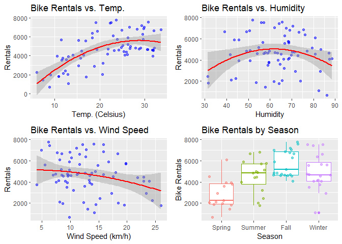
Next we look at scatter plots of total daily rentals vs. the numeric weather measures with quadratic regression lines over-layed. Additionally, we create box plots by season to visually inspect the differences in bike rentals by season.
###
# Create scatter plots for bike rentals vs. our numeric variables and box plots
# for bike rentals by season.
###

plot5 <- ggplot(bikeTrain, aes(x=temp*41, y=cnt)) +
  geom_point(color="blue", alpha=0.5) +
  geom_smooth(method = 'lm', formula='y ~ poly(x, 2)', color="red") +
  xlab("Temp. (Celsius)") +
  ylab("Rentals") +
  ggtitle("Bike Rentals vs. Temp.")

plot6 <- ggplot(bikeTrain, aes(x=hum*100, y=cnt)) +
  geom_point(color="blue", alpha=0.5) +
  geom_smooth(method = 'lm', formula='y ~ poly(x, 2)', color="red") +
  xlab("Humidity") +
  ylab("Rentals") +
  ggtitle("Bike Rentals vs. Humidity")

plot7<- ggplot(bikeTrain, aes(x=windspeed*67, y=cnt)) +
  geom_point(color="blue", alpha=0.5) +
  geom_smooth(method = 'lm', formula='y ~ poly(x, 2)', color="red") +
  xlab("Wind Speed (km/h)") +
  ylab("Rentals") +
  ggtitle("Bike Rentals vs. Wind Speed")

plot8 <- ggplot(bikeTrain, aes(x=season, y=cnt, color=season)) +
  geom_boxplot() +
  geom_jitter(alpha=0.5) +
  xlab("Season") +
  ylab("Bike Rentals") +
  ggtitle("Bike Rentals by Season") +
  theme(legend.position="none")

plot_grid(plot5, plot6, plot7, plot8)

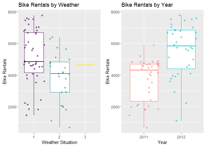
Finally, we examine the distributions of bike rentals by weather situation and year. We can tell if the distribution of bike rentals varies by weather conditions or by year.
###
# Create box plots of bike rentals by weather situation and year.
###

plot9 <- ggplot(bikeTrain, aes(x=weathersit, y=cnt,
                                        color=weathersit)) +
  geom_boxplot() +
  geom_jitter(alpha=0.5) +
  xlab("Weather Situation") +
  ylab("Bike Rentals") +
  ggtitle("Bike Rentals by Weather") +
  theme(legend.position="none")

plot10 <- ggplot(bikeTrain, aes(as.factor(yr+2011), cnt,
                                color=as.factor(yr+2011))) +
  geom_boxplot() +
  geom_jitter(alpha=0.5) +
  xlab("Year") +
  ylab("Bike Rentals") +
  ggtitle("Bike Rentals by Year") +
  theme(legend.position="none")

plot_grid(plot9, plot10)

We now have an idea of how our predictive features relate to the number of bike rentals, so we are ready to move onto modeling.
Modeling
We want to predict bike rental demand in a given day conditional on weather-related variables, the season, and the year. These can be known a priori (assuming a weather forecast for the next day is very accurate). We will try linear and ensemble modeling approaches.
# Set the parameters for repeated k-folds CV.
k <- 5
repeats <- 3

# Create a trainControl object for repeated k-folds CV.
trCntrl <- trainControl(method="repeatedcv", number=k, repeats=repeats)
We are doing 5-folds CV with 3 repeats.
Linear Models
Linear regression models a dependent variable as a function of a set of independent variables that is linear in its parameters. The most widely-known linear regression technique is ordinary least squares (OLS), which assumes normally distributed errors. OLS is a special case of the generalized linear model (GLM), which allows for the errors to follow non-normal distributions. We will try both an OLS model and a GLM, with the same variables and transformations.
Linear Model 1 (OLS)
For our first model, we are assuming the number of bike rentals has quadratic relationships with temperature, wind speed, and humidity, with seasonal effects, and a linear trend for year. The linear trend of year will probably perform particularly poorly for extrapolation. As the bike rental company is around longer, their rate of yearly growth will decrease as they approach market saturation. The model is shown below.
# of rentalsi = β0 + β1tempi + β2tempi2 + β3wind speedi + β4wind speedi2 + β5humidityi + β6humidityi2 + β7Summeri + β8Falli + β9Winteri + β10yeari + ϵi
where
ϵi ∼ N(0, σ2)
Thus, our model for the distribution of bike rentals in a day for Tuesday is:
# of rentalsi ∼ N(μi = β0 + Σj = 110βjxj, i, σ2)
where xi is the ith variable in the regression model.
We will refer to this model as the OLS model.
# Evaluate a linear model of the specified form in repeated k-folds CV and fit
# it to the training set.
linMod1 <- train(
  cnt ~ temp + I(temp^2) + windspeed + I(windspeed^2) + hum + I(hum^2)
  + season + yr,
  data=bikeTrain,
  method="lm",
  trControl=trCntrl
  )
Linear Model 2 (Poisson Regression)
In our second linear model, poisson process is applied to the same combination of variables and any quadratic effects.Poisson regression model is one of generalized linear models (g(μ) = β0 + β1x1 + β2x2 + … + βpxp where μ denotes the mean corresponding to x sets.) for modeling count data. Because bike rentals being a count and our count occurs in a set amount of time (a single day), it is reasonable to use poisson regression for modeling here. . Our model for the λ parameter of the Poisson distribution is:
λi = β0 + β1tempi + β2tempi2 + β3wind speedi + β4wind speedi2 + β5humidityi + β6humidityi2 + β7Summeri + β8Falli + β9Winteri + β10yeari + ϵi
where
ϵi ∼ N(0, σ2)
Thus, our model for the distribution of bike rentals in a day for Tuesday is:
# of rentalsi ∼ Poisson(λi = β0 + Σj = 110βjxj, i)
We will refer to this model as the Poisson Regression model.
# Evaluate a linear model of the specified form in repeated k-folds CV and fit
# it to the training set.
linMod2 <- train(
  cnt ~ temp + I(temp^2) + windspeed + I(windspeed^2) + hum + I(hum^2)
  + season + yr,
  data=bikeTrain,
  method="glm",
  family="poisson",
  trControl=trCntrl
  )
Tree-based Ensemble Models
Tree-based ensemble methods are very popular in applied machine learning due to their ability to model non-linear and interaction effects without explicit direction to do so. Here we try the two most popular ensemble methods: random forests and gradient boosted trees. We also perform a grid search in our repeated k-folds CV to tune our models for the best hyper-parameters.
Random Forest
Random forests create B boostrapped samples and fit trees to each of the boostrapped samples. At each split in each tree, only a random subset of variables are considered. Both steps push the trees to grow independently on one another. For regression, the predictions of trees are averaged to get the final predicted value. For classification, the majority vote of class membership is generally used to predict the class.
The combination of pushing the trees to grow independently and averaging should lower the variance of our prediction. Given the mean squared error can be decomposed into the squared bias plus the variance of the model, this will hopefully decrease the MSE (if the reduction in variance is greater than the increase in squared bias).
We now fit our random forest model, hereafter referred to as the Random Forest model, trying 100, 500, and 1000 trees.
# Perform the grid search through repeated CV.
rfFit <- train (
  cnt ~ temp + windspeed + hum + season + yr,
  data=select(bikeTrain, -"weekday"),
  method="rf",
  preProcess= c("center", "scale"),
  trControl = trCntrl,
  tuneGrid=expand.grid(mtry=c(100, 500, 1000))
  )
Boosted Trees
Boosting is one of tree based statistical ensemble learning methods for regression or classification. Like other tree based methods, boosted tree involves in splitting predictor space into regions. But it has also some unique features: the tree growth is sequential and slow, which means each tree is modified based on previous one. Three parameters are used to tune boosting process: number of trees B, shrinkage parameter lambda bad split number d which control the complexity of boosted ensembles. Boosted tree tends to decrease bias.
Now we can choose our hyper-parameters through repeated k-folds CV and fit our model, which we refer to as the Boosted Trees model.
# Set grid of tuning parameters to try.
gbmGrid <- expand.grid(
  interaction.depth=c(1, 4, 6),
  n.trees=c(100, 500),
  shrinkage=c(0.01, 0.1),
  n.minobsinnode=c(3, 10)
)

# Perform the grid search through repeated CV.
gbmFit <- train (
  cnt ~ temp + windspeed + hum + season + yr,
  data=select(bikeTrain, -"weekday"),
  method="gbm",
  preProcess= c("center", "scale"),
  trControl = trCntrl,
  tuneGrid=gbmGrid
  )
Comparing the Models
With the repeated k-folds CV completed and our models fit, we can evaluate their performance in CV and on the withheld testing set.
Let’s evaluate their repeated k-folds CV performance first.
# Create a list of models and vector of model names.
modelList <- list(linMod1, linMod2, rfFit, gbmFit)
modelNames <- c("OLS", "Poisson Regression", "Random Forest", "Boosted Trees")

###
# Extract model performances and put them in a summary table.
###

cvRMSE <- unlist(
  sapply(
    sapply(
      sapply(modelList, FUN="[", "results"),
      FUN=filter, RMSE==min(RMSE)),
    FUN="[", "RMSE"
    )
  )

cvMAE <- unlist(
  sapply(
    sapply(
      sapply(modelList, FUN="[", "results"),
      FUN=filter, MAE==min(MAE)),
    FUN="[", "MAE"
    )
  )

cvRsquared <- unlist(
  sapply(
    sapply(
      sapply(modelList, FUN="[", "results"),
      FUN=filter, Rsquared==max(Rsquared)),
    FUN="[", "Rsquared"
    )
  )

# Create a data.frame of model performances.
cvPerformance <- data.frame(
  Model=modelNames,
  RMSE=cvRMSE,
  Rsq=cvRsquared,
  MAE=cvMAE
)

# Extract the best model's name and RMSE.
bestModelCV <- cvPerformance %>%
  mutate(Model = modelNames) %>%
  filter(RMSE == min(RMSE)) %>%
  select(Model, RMSE)
# Save the model name and RMSE to 2 decimal places as vairables.
bestModelNameCV <- bestModelCV$Model
bestRMSECV <- round(bestModelCV$RMSE, 2)

# Display the table in a neat format.
knitr::kable(
  cvPerformance,
  digits=2,
  caption="Table 3: Repeated k-folds CV Performance Summary",
  col.names=c("", "RMSE", "Rsquared", "MAE")
)
| RMSE | Rsquared | MAE | |
|---|---|---|---|
| OLS | 757.79 | 0.83 | 600.23 |
| Poisson Regression | 644.74 | 0.87 | 501.72 |
| Random Forest | 837.04 | 0.79 | 648.86 |
| Boosted Trees | 653.82 | 0.87 | 502.69 |
Table 3: Repeated k-folds CV Performance Summary
The best performing model in repeated k-folds CV is the Poisson Regression with an RMSE of 644.74. Usually, we would pick the best performing model here to test on the testing data, but we will compare them all this time.
Now let’s look at their test set performance.
evaluatePeformance <- function(model, dataEval, target){
  ###
  # This function takes in a fit model, testing data (tibble), and a target
  # variable (string) and returns the performance.
  ###
  preds <- predict(model, newdata=dataEval)
  return(postResample(preds, pull(dataEval, target)))
}

# Get the test set performances.
testPerformances <- sapply(
  modelList, FUN=evaluatePeformance, dataEval=bikeTest, target="cnt"
  )
# Rename the columns with the model names.
colnames(testPerformances) <- modelNames

# Convert the table to data.frame.
testPerformances <- as.data.frame(t(testPerformances))

# Extract the best model's name and RMSE.
bestModel <- testPerformances %>%
  mutate(Model = modelNames) %>%
  filter(RMSE == min(RMSE)) %>%
  select(Model, RMSE)
# Save the model name and RMSE to 2 decimal places as vairables.
bestModelName <- bestModel$Model
bestRMSE <- round(bestModel$RMSE, 2)

# Display the table in a neat format.
knitr::kable(
  testPerformances,
  digits=2,
  caption="Table 4: Test Set Performance Summary",)
| RMSE | Rsquared | MAE | |
|---|---|---|---|
| OLS | 845.71 | 0.84 | 681.96 |
| Poisson Regression | 751.89 | 0.86 | 609.47 |
| Random Forest | 948.53 | 0.76 | 730.53 |
| Boosted Trees | 823.44 | 0.82 | 638.08 |
Table 4: Test Set Performance Summary
The best performing model on the testing set is the Poisson Regression with an RMSE of 751.89.